Online testing sample calculator
I built an online sample testing calculator. It calculates required sample sizes, estimated time to finish and statistical significance of tests. This post will explain how it works and how to use it.
Published on: December 06, 2017.
Last revised on: January 7, 2024.
First published at: https://www.automacaodedados.com.br/en/stories/calculadora-de-significancia-estatistica-para-testes-ab/
The series on statistics for testing published on this blog presented several inferential statistics concepts that are used when testing with samples. This calculator will use everything that was presented on that series.
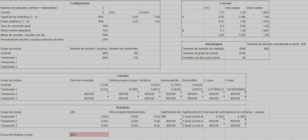
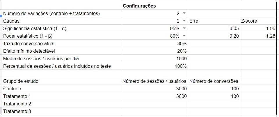
Settings
This is the editing section. Options are:
Number of variations (control + treatments): number of slices from the sample, including the control group;
Tails: number of tails. This option configure α (alpha) to be distributed along the tails of the distribution. In practice, defines if researchers are expecting better or worse results when applying the treatment. If there are two tails, alpha will become α / 2;
Statistical significance (1 - α): confidence interval associated with the result, or the probability of correctly rejecting the null hypothesis;
Statistical power (1 - β): probability that the expected result will be found. In statistical terms is the probability of correctly accepting the alternate hypothesis. Most calculators and testing tools use 80% statistical power (or 20% probability of false negative errors). β is the Greek letter that represent beta;
Current conversion rate: average conversion rate;
Minimum detectable effect: minimal amount of difference between study groups that is expected. Useful to ignore small differences, which probably aren’t relevant or costly to implement;
Average daily number of sessions / users: this average is from people that visit pages that are being testes. This will be used to estimate the amount of days which the test should run;
Percentage of sessions / users to be included in the test: percentage of traffic participating from the test.
Z-score and Error options are used for the remaining calculations. Error subtracts alpha from the statistical significance using the equation 1 - (1 - α), where 1 - α is statistical significance. Alpha and beta z-scores are used to calculate the sample size.
For each part of the sample, options are:
Number of sessions / users: number of visitors that were included in each testing variation. Note that it is up to the researcher to measure using users, sessions or visits. Testing tools usually go with sessions, but depending on each business the number of sessions and the number of users can be very different from one another;
Number of conversions: number of conversion events in each variation.
This calculator accepts up to 4 variations (control + three treatments), but if tests have less than four, just configure the number of variations and access / conversion data accordingly, leaving empty the fields that aren’t required.
Z-scores
This z-scores table is used to calculate the sample size with one and two tails. Sample testing tools and calculators don’t show this table. It is used to look up the respective z-scores for configured statistical significance and statistical power.
Sample size
Sample size is calculated using the equation numerator * (σ / (p * effect)), where numerator is 2 * (α + β)², p is the current conversion rate and effect is the minimum detectable effect, or the size of the difference that the researcher is expecting between control and treatment groups. Letter σ is the sample standard deviation. The numerator is based on Lehr's equation, an estimator of sample size, and most tools simply assume the number 16. In order for numerator to be 16, α should be 0.05 and β should be 0.2. In other words, statistical significance should be 95% and statistical power should be 80%. The exact numerator when using these values for alpha and beta is 15.68. This number is, then, rounded to 16. This calculator estimates the numerator without using the 16 rule, as it is known, which produces sample sizes that are different from other calculators and tools.
Alongside sample size by variation the sample size used in the test is shown. This number varies according to the traffic that is participating from the test.
The size of the study group is the product of sample size and number of variations. For cases when not using 100% of traffic for testing, it is used the equation ((((1 - traffic) * sample) + (sample * traffic)) * variations) - 1, where traffic is the percent of traffic to participate from the test, sample is the sample size per variation and variations is the number of testing variations (control + treatments). Subtracting 1 at the end approximates the amount of traffic with the sum from each variation.
Estimated number of days for testing is a division between total sample and average daily number of visitors, considering all traffic that will be used for testing. Note that this estimate can differ by quite a lot from other calculators. VWO's test duration estimator, for instance, estimate a total of 37 days to run the test considering these settings:
Estimated existing conversion rate: 30%;
Minimum improvement in conversion rate you want to detect: 10%;
Number of variations / combinations (including control): 2;
Average number of daily visitors: 1000;
Percent visitor included in test: 20%.
This calculator estimates 49 days to test with two tails and 29 with one tail, using the same options. This happens because the way the numerator is calculated, not using the 16 rule, and for the fact that the number of tails is assumed at VWO’s calculator.
Calculations
After setting up the calculator, equations will be executed and the answers will be obtained. These calculations are:
Conversion rate: proportion of the sample that triggered the conversion event. The equation used was p = s / t, where p is proportion, s is the number of conversions and t is the sample size for each variation;
Difference from the control group: conversion rate difference between treatments and control. The equation used was (p1 / p0) - 1, where p1 is the proportion for the treatment group, p0 is the proportion for the control group and -1 is a transformation applied to the inverse of the quotient (the result of a division). This transformation represent the difference between conversion rates;
Variance: measure of spread throughout the distribution. The equation used was σ² = p * (1 - p), where σ² is the variance. It is calculated by multiplying a proportion and its compliment. Greek letter σ is called sigma;
Standard deviation: square root of variance. Squaring the variation is used to better represent the spread of data along a distribution. Equation used is σ = √σ², where σ is the standard deviation;
Standard error: similar to the standard deviation, but spread is calculated compared to the population mean. This is particularly useful to determine a standard deviation measure when two or more samples are being studied, which is the case with tests with online samples. For standard errors, averages from all variations are used to calculate a single average, which is then used to calculate the deviation. Equation used is σx̄ = σ / √n, where σx̄ is the standard error and n is the sample size. x̄ is the sample mean;
Z-score: number of standard deviations compared to the mean. The z-score traditional equation is z = (x - μ) / σ, where z is the z-score, x is an individual proportion (in this case, the value associated with p) and μ is the population mean. Since the population mean is unknown, there is more than one study group and the measures of deviation must be standardized to compare across normal distributions, the following equation is used: (p1 - p0) / √(σx̄0² + σx̄1²), where p1 is the proportion associated with treatment group, p0 is the proportion associated with control group, σx̄0² is the squared standard error associated with control group and σx̄1² is the squared standard error associated with treatment group;
P-value: assuming the null hypothesis, it is the probability of observing an extreme event. In other words, the probability that an anomaly will be observed if no changes were made to the study group. The hypothesis is that this probability is very low, so if this number is small enough, chances are that the anomaly was not by chance and was indeed the result of a treatment gave to one or more samples by researches. The equation is 1 - NORMDIST(ABS(z)), where NORMDIST is the function that calculates a cumulative normal distribution on Google Sheets. Since proportion is a continuous variable (can assume infinite values), the function that explains this variable is a cumulative one. ABS is the module function on Google Sheets, it transforms a number into its positive counterpart, since p-value is a number between 0 and 1. The calculation of z inside a normal distribution corresponds to an area that is covered by z. P-value is the opposite of this number and represent an area that goes from one of the tails of a normal distribution to the value assumed by p-value, hence subtracting 1 at the beginning of the equation.
This section display the end results from the calculations. It shows α and β, if the reuslt is statistically significant and the confidence interval. For α, it is applied Bonferroni’s correction when there are more than two testing variations. For each variation added in a multivariate test, chances of a type I error (false positive) increase. Bonferroni’s correction is one of many ways to control for increase α values, and the equation is α / variations, where variations is the number of testing variations (control + treatments). Bonferroni’s correction is said to be conservative since decrease α, requiring bigger sample sizes to get statistical significance.
To end, the calculator show if it is possible to stop the test or not. The equation check the number of variations to be tested and if two conditions are met:
If the total size of the study group that participated in the test is greater than or equal to the calculated sample size;
If all treatments have statistical significance greater than or equal to what is configured.
If it is a multivariate test, statistical significance is checked after Bonferroni’s correction.
Further reading
There are many online calculators for sample sizes, statistical significance and test duration. Each calculator assume some values to abstract some of the complexity related to statistics. This calculator works differently, since no values are assumed.
The following calculators were used as reference to build this one:
In case you need a quick recap on inferential statistical concepts, check out the statistical series here on this blog.
Let’s calculate statistical significance, sample size and test duration!


